
Working with dates is an essential skill for anyone working in Excel. For example, in project management, you may need to be able to work with date duration. In finance and accounting, you’ll often need to aggregate data across different periods of time. In this tutorial, you’ll learn how to get the quarter from a date in Excel.
A quarter is a time period of three months, meaning that there are four quarters in each year. Calendar quarters start in January, while financial quarters generally start in April.
| Quarter | Calendar Quarters Date Range | Financial Quarters Date Range |
|---|---|---|
| Quarter 1 | January 1 to March 31 | April 1 to June 30 |
| Quarter 2 | April 1 to June 30 | July 1 to September 30 |
| Quarter 3 | July 1 to September 30 | October 1 to December 31 |
| Quarter 4 | October 1 to December 31 | January 1 to March 31 |
By the end of this tutorial, you’ll have learned the following:
- How to get the quarter from a date in Excel
- How to get the year and quarter from a date in Excel
- How to get the financial (or fiscal) quarter from a date in Excel
How to Get a Quarter Number from a Date in Excel
How can you get the quarter from a date in Excel?
To get the quarter from a date in Excel, use the following function: =ROUNDUP(MONTH(A2)/3, 0). The function will divide the month number by 3 and round the value up to its nearest whole number.
Let’s take a look at how this function works:
= MONTH(A2)Excel first gets the month number from a date, which returns a number from 1 through 12. For example, the date April 2, 2023, would return 4.
= MONTH(A2) / 3We divide that number by 3, which returns a number between 0 and 4. For example, using April 2, 2023, Excel would return 4 / 3, which is equal to 1.33.
= ROUNDUP(MONTH(A2) / 3, 0)Finally, we round the number up to its nearest whole number, which returns a number between 1 and 4. Using our previous example, Excel would round 1.33 up to 2.
Let’s take a look at a step-by-step example of how to get the quarter from a date in Excel.
Step 1: Load your data in Excel
In our sample workbook, we have 5 different dates from different periods of the year. In the second column, we want to get the quarter number for each date.
Step 2: Divide your date’s month by 3 and round up
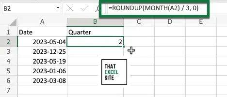
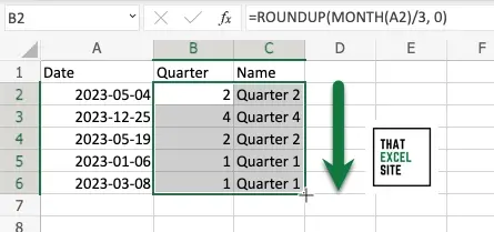
We use the formula =ROUNDUP(MONTH(A2)/3, 0) to get the number for the quarter of the first date. When you hit the Enter key, the formula evaluates and Excel returns the number matching the date’s quarter.
Step 3: Drag the fill handle down to get the quarter for each date
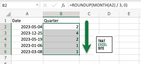
By clicking and dragging the fill handle all the way down, Excel copies the formula for the remaining dates in your dataset. When you let go of the mouse, Excel will return the quarter number for each date.
In the following section, you’ll learn how to get and customize the quarter name for a date in Excel.
How to Get a Quarter Name from a Date in Excel
In the previous section, you learned how to get the quarter number from a given date. In many cases, however, you’ll want to customize the way in which the quarter is displayed. For example, the label Quarter 3 is much more intuitive and understandable than simply “3”. Being able to convert the quarter number to a label works by concatenating a text label with the number of the quarter.
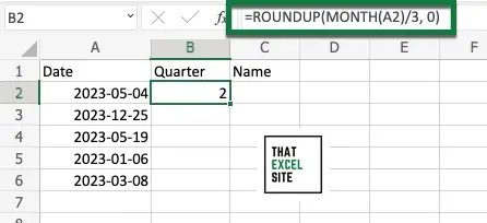
Step 1: Load your data in Excel
In our sample workbook, we have 5 different dates from different periods of the year.
Step 2: Divide your date’s month by 3 and round up
We use the formula =ROUNDUP(MONTH(A2)/3, 0) to get the number for the quarter of the first date. When you hit the Enter key, the formula evaluates and Excel returns the number matching the date’s quarter.
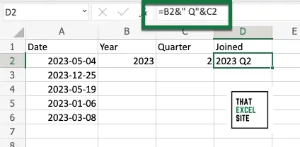
Step 3: Join the quarter number with the text you want to use
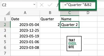
In the example above, we use the ampersand sign to concatenate the label "Quarter " and the quarter number. You can use whatever label you want. Keep in mind, Excel won’t automatically include a space in your text. If your text is meant to have a space, make sure you insert it in the label string.
Step 4: Drag the fill handle down to get the quarter for each date
By clicking and dragging the fill handle all the way down, Excel copies the formula for the remaining dates in your dataset. When you let go of the mouse, Excel will return the quarter name for each date.
How to Get the Year and Quarter from a Date in Excel
In many cases, you’ll want to get the both the year and the quarter from a date in Excel. This can be helpful you want to easily sort values broken out not just by their year or quarter, but by both. In this case, we’ll convert the year and the quarter into a string of text to be able to customize the output however we may want to.
Step 1: Load your data in Excel
In our sample workbook, we have 5 different dates from different periods of the year.
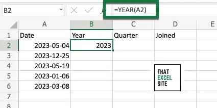
Step 2: Get the year from the date in Excel
First, we’ll get the year from a date in Excel so that we can join the year with the quarter. While we could do all this in a single column, breaking it out into single steps lets you see what’s going on under the hood.
Step 3: Divide your date’s month by 3 and round up
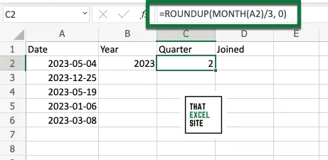
We use the formula =ROUNDUP(MONTH(A2)/3, 0) to get the number for the quarter of the first date. When you hit the Enter key, the formula evaluates and Excel returns the number matching the date’s quarter.
Step 4: Combine the Year and Quarter Into Text
Combine the year and quarter numbers into a string of text that makes the values more legible.
Step 5: Drag the fill handle down to get the quarter for each date
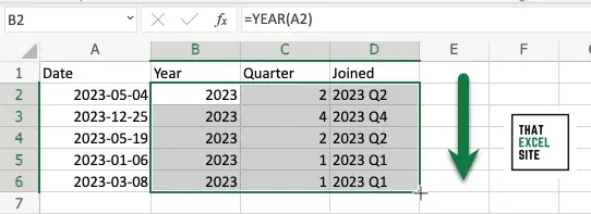
By clicking and dragging the fill handle all the way down, Excel copies the formula for the remaining dates in your dataset. When you let go of the mouse, Excel will return the year and quarter numbers for each date.
How to Get the Fiscal Quarter from a Date in Excel
Step 1: Load your data in Excel
In our sample workbook, we have 5 different dates from different periods of the year. In the second column, we want to get the quarter number for each date.
Step 2: Use the CHOOSE() function to return the quarter number
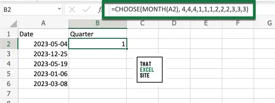
We use the formula =CHOOSE(MONTH(A2), 4, 4, 4, 1, 1, 1, 2, 2, 2, 3, 3, 3) to get the number for the quarter of the first date. When you hit the Enter key, the formula evaluates and Excel returns the number matching the date’s quarter.
The way that this function works is by providing twelve different options Excel can choose from. If the MONTH(A2) function returns, say a 1, it will choose the first item. Similarly, if the function returns a 7, it will return the seventh item.
Step 3: Drag the fill handle down to get the quarter for each date
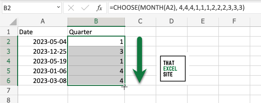
By clicking and dragging the fill handle all the way down, Excel copies the formula for the remaining dates in your dataset. When you let go of the mouse, Excel will return the fiscal quarter number for each date.
Conclusion
Being able to analyze and summarize your Excel data by quarter is an incredibly useful skill to have. For example, you may need to use these skills in developing financial reports or being able to track performance over a period of time. In many cases, however, you’ll only be given a date, rather than a quarter itself.
In this tutorial, you learned how to get the quarter from a date in Excel. You first learned how to get just the quarter number, by making use of the ROUNDUP() function and the MONTH() function. Then, you learned how to label the quarter as a text string by using the ampersand concatenate operator.
From there, you learned how to get the year and quarter for a given date, by combining what you learned with the YEAR() function. Finally, you learned how to customize quarters to different start months, such as financial quarters, by using the CHOOSE() function.
Additional Resources
To learn more about related topics, check out the tutorials below: