Excel SUMIF(): How to Use the Excel SUMIF() Function

The Excel SUMIF() function is a logical function that is used to sum the number of cells that meet specific criteria. For example, the function can be used to add up values for only specific cities that appear in a list of sales. In this tutorial, you’ll learn how to use the Excel SUMIF() function and how to customize it to meet your needs. You will learn all the basics of the function and even dive into some advanced uses of the function.

By the end of this tutorial, you’ll have learned:

• How to understand and how to use the Excel SUMIF() function
• How to resolve common problems that occur when using the Excel SUMIF() function
• What some of the best practices are when working with the SUMIF() function
• How to dive deeper into the function using custom use cases of the function

Understanding the Excel SUMIF() Function

Let’s take a look at the Excel SUMIF() function and its arguments to better understand how to use it:

=SUMIF(range, criteria, [sum_range])

As you can see from the code block above, the function takes three arguments. Let’s take a closer look at them in the table below:

Argument	Description	Required?
range=	The range of cells to apply the condition to	Yes
criteria=	The condition to apply, including any of the logical operators that may be required	Yes
sum_range=	The range of cells to add up. If empty, Excel adds up the values in the range= argument.	No

The criteria can be thought of as either logical, wildcards, or partial matches. This is extremely powerful, allowing you to customize the function quite a bit. For example, you can search for a cell that contains an exact string, or even just a partial string. For example, you can use wildcard operators to search for a text string starting with “South”, but could be either “South-West” or “South-East”.

Let’s take a look at how some of these criteria work in the Excel SUMIF() function:

1. Logical operators can check for a logical condition, such as if an item is equal to, less than, and more. These operators include: <, >, <=, >=, and =.
2. Wildcard operators let you use characters to represent different types of strings. For example, the ? character represents any single character. The * character, on the other hand, represents any number of any character.

Now that we’ve covered a lot of the theory of the function, let’s dive into an example of how you can use the function.

How to Use the Excel SUMIF() Function

Using the Excel SUMIF() function can feel a little unnatural at first. This is especially true because there are a number of different options for how to search for different criteria. In this section, we’ll take a look at a simple example first and then dive into some other use cases of how to apply different criteria.

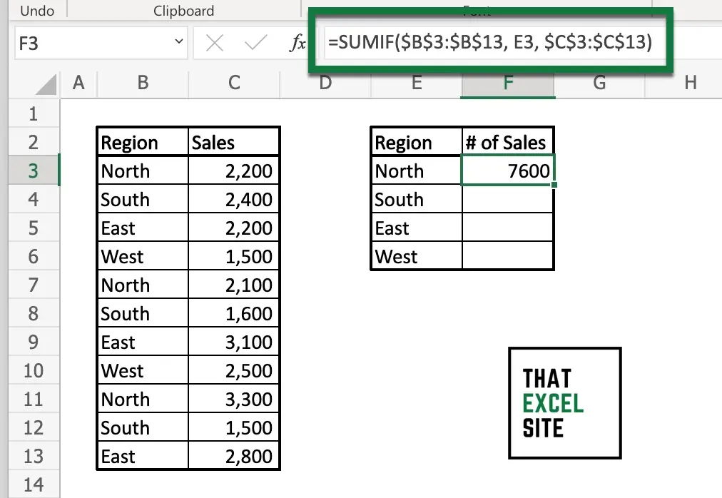
Let’s break down what we’re doing in the example above. We use the formula below to add up the sales for any value where the region is equal to North:

=SUMIF($B$3:$B$13, E3, $C$3:$C$13)

In the function above, we use the following values:

1. The range is $B$3:$B$13. This means that Excel searches for the criteria in this range of data.
2. The criteria is E3, meaning that we’re searching for the value North.
3. The sum range is $C$3:$C$13, meaning that the values in these cells will be added up if the record has a corresponding matching condition.

In order to apply this to all of the different regions, we can drag down the fill handle, as shown in the image below:

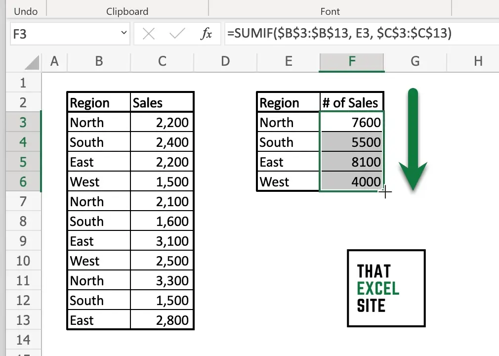
By clicking and dragging the fill handle (the little crosshair in the bottom right of a cell) all the way down through the rest of the data, Excel will copy the formula for all remaining data. When doing this, be mindful to use absolute references for both of the ranges. Without this, Excel would change the references when dragging the values down.

Now that we’ve walked through a simple example, let’s take a look at some of the different criteria options available.

Understanding Different Criteria Options in the Excel SUMIF() Function

The Excel SUMIF() function provides a large variety of criteria options. Earlier, you learned that you can use logical and wildcard operators. This can include dates and cell references, as well.

The table below breaks down the different options available to you in searching for different criteria in the SUMIF() function:

Criteria Logic	Excel Criteria
Cells equal to “North”	“North”
Cells not equal to “North”	“<>North”
Cells starting with “North”	“North*”
Cells ending with “West”	“*West”
Cells greater than 1000	“>1000”
Cells greater than or equal to 1000	“>=1000”
Cells less than 1000	“<1000”
Cells less than or equal to 1000	“<=1000”
Cells equal to 1000	1000
Cells less than the value in A2	“<“&A2
Cells greater than today’s date	“<“&TODAY()
Cells not equal to today’s date	“<>”&TODAY()

While a lot of these probably make sense, some of them may stick out as odd. For example, when you’re using a function or a cell reference in your criteria, be sure to wrap the operator in a string. When you do this, you need to concatenate the string using the ampersand operator.

In the following section, you’ll learn how to tackle common problems when working with the SUMIF() function.

How to Use Excel SUMIF() to Add Values Not Equal to a Value

Say that we want to add up the sales values based on a value not being equal to a particular value in the region range. The SUMIF() function allows this, since it allows us to pass in the optional sum range argument.

Let’s take a look at what this looks like in Excel:

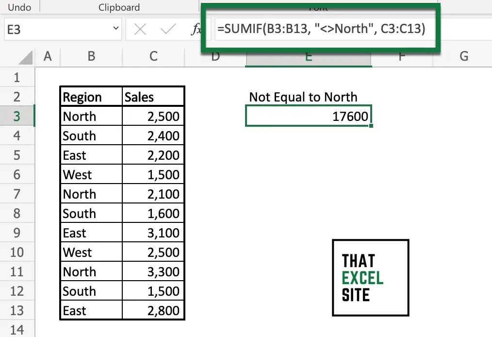
In the example above, we’re using the following formula:

=SUMIF(B3:B13, "<>North", C3:C13)

This formula instructs Excel to search for the criteria in the range B3:B13. We’re using the condition of "<>North", which indicates that we’re looking for values that aren’t equal to North. Keep in mind that this criteria argument is case-insensitive, meaning that it will also find cells equal to north and other permutations. Finally, we use the C3:C13 range as the sum range argument, which instructs Excel to add only the values that meet the condition.

To learn more about how to use the SUMIF() and SUMIFS() functions to add values that aren’t equal to a value check out this guide.

How to Use Excel SUMIF() to Add Values Greater Than a Value

We can use the function to add values that are greater than a value by using the criteria of ">"&value. Note that we’re wrapping the condition in double quotes and then joining it with the value that we’re comparing to.

Let’s see how we can use Excel to add values that are greater than a value:

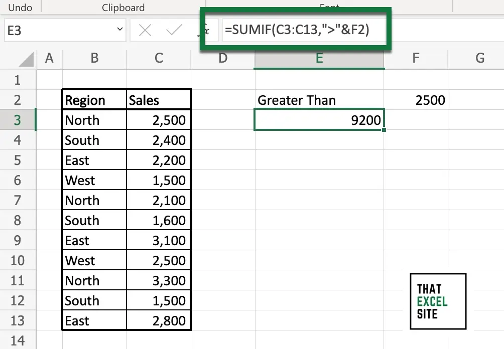
In the example above, we used the following formula:

=SUMIF(C3:C13, ">"&F2)

The formula adds up the values in the range C3:C13 if they are greater than the value in cell F2 (which, in this case, is 2500). Since we’re adding the same range as the criteria range, we can omit the third argument (the sum range).

How to Use Excel SUMIF() with Less Than Conditions

Similar to adding values that are less than a value, we can also use the SUMIF() function to add values that are less than or equal to a value. In order to do this, we only need to change the operator to include cells that are equal to or less than a value.

We can sum values that are less than or equal to a value by using the following formula:

=SUMIF(C3:C13, "<="&F2)

Let’s take a look at an example of how to add values that are less than or equal to a value using the SUMIF() function:

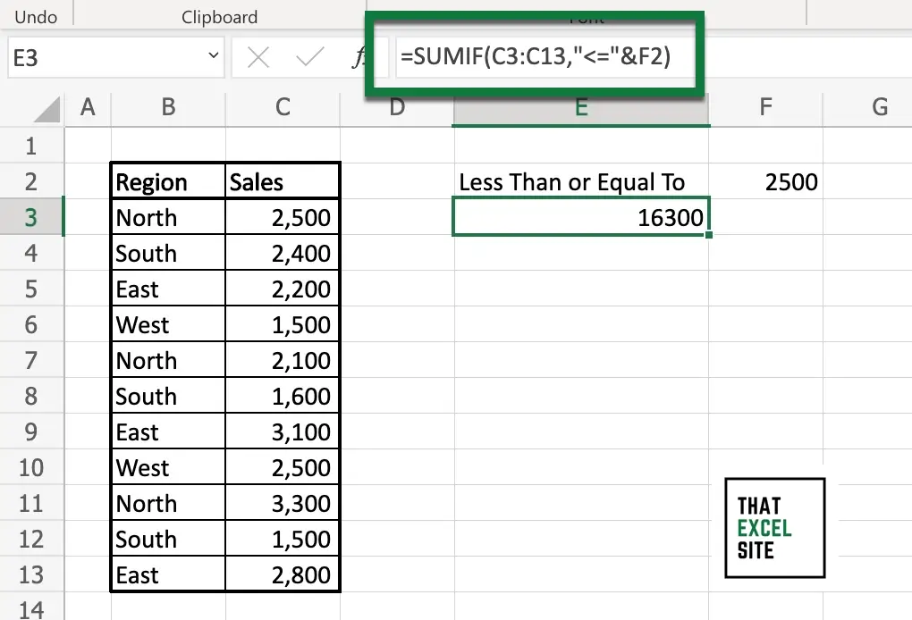
In the example above, we modified the SUMIF() function to add values that are less than or equal to a certain value. With this, you can add cells that don’t meet a specific quote, for example.

How to Use Excel SUMIF() with Containing Partial Text Matches

We can also use Excel to add values that contain partial text matches, or even ones that start or end with a particular text.

Being able to add values that contain partial text can be done by using the wildcard operator *. Excel uses two wildcard operators: ? which checks for only a single character and * which checks for any number of characters.

In order to use the Excel SUMIF() function to add cells containing partial matches, we can use the following formula:

=SUMIF(criteria_range, "*"&text&"*", sum_range)

Let’s see what this looks like by taking a look at a practical example:

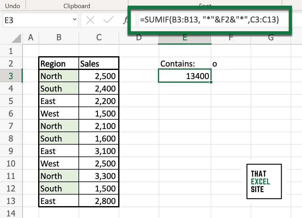
In the example above, we have our text in range B3:B13 and the values we want to add up in range C3:C13. Specifically, we’re looking for cells that contain the string "o", which we’re storing in cell F2. We can use the following formula to add cells that contain the partial text:

=SUMIF(B3:B13, "*"&F2&"*",C3:C13)

Notice that we’re wrapping the wildcard operator in double-quotes. This is necessary so that Excel doesn’t throw an error. If we were hard coding the condition (rather than using a cell reference), we could use "*o*". However, this doesn’t allow our formula to be dynamic, such as if we wanted to modify the text in cell F2.

How to Sum Only Positive or Negative Numbers with Excel SUMIF()

Because the function can be used to add values conditionally, we can easily add a condition to the function to include only positive numbers. This can be incredibly helpful if you are trying to add only incomes over a transaction sheet that also includes spending.

Let’s see how we can write a formula to add only numbers above zero:

=SUMIF(range, ">0")

Now that you have the formula to work with, let’s see what this looks like in action by using a hands-on example:

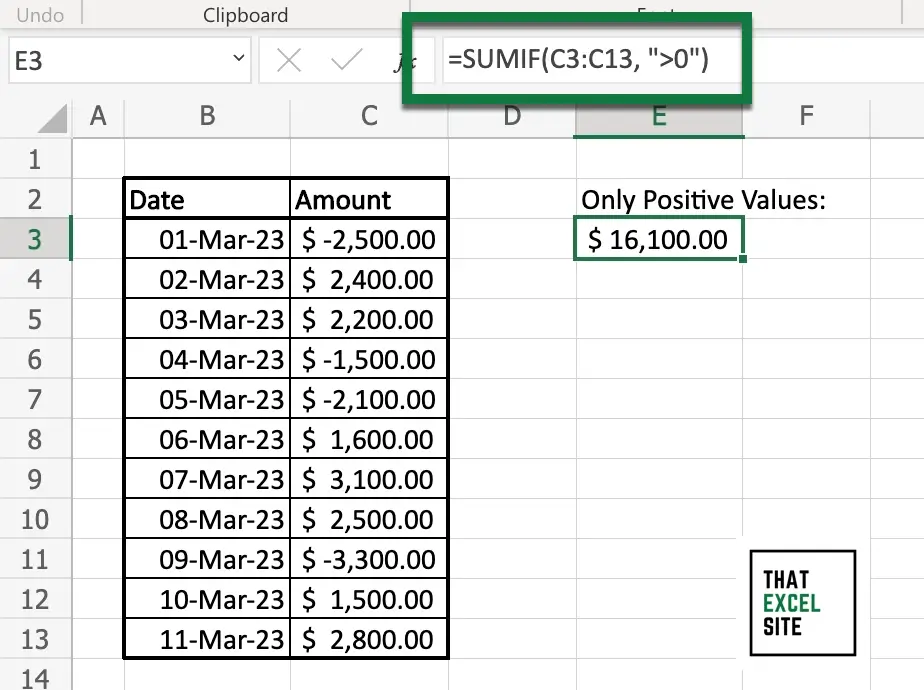
In the example above, we’re adding together only positive numbers. Because the criteria range is the same as our sum range, we can safely omit the third optional argument. Because our condition excludes any negative values, we’re summing up only positive values within the range.

How to Use Excel SUMIF() Before a Specific Date

We can also use the Excel SUMIF() function to add values only before (or after) a specific date. In order to do this, we can use the SUMIF() function and pass in the date range as the criteria range, the condition of "<"&date, and the values as our sum range.

Let’s take a look at an example of what this looks like:

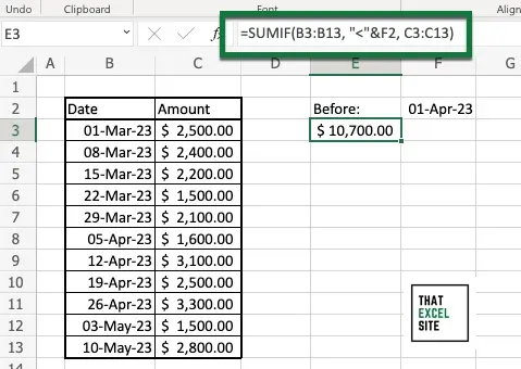
We use the following formula to sum values before a specific date:

=SUMIF(B3:B13, "<"&F2, C3:C13)

Note that we’re wrapping the less than operator in double quotes and then concatenating the date to it. This allows us to avoid any errors. Because Excel uses numbers to store dates, this process is actually the same as using the SUMIF() function to add values less than a certain value.

How to Use SUMIF() With OR Logic Using Dynamic Arrays

Dynamic array functions allow for you to simplify your code and make it more dynamic at the same time. We can use the SUMIF() function with OR logic by passing an array of values into the SUMIF() function. We create these arrays by passing the values into curly braces. If we wanted to add cells where the region was equal to North or South, we could write {"North", "South"}.

Let’s see how we can use array functions to calculate SUMIF() with OR logic. Use the formula below:

=SUMIF(B3:B13, {"North", "South"})

Let’s see what happens when we use this function in Excel to add cells meeting multiple conditions with OR logic:

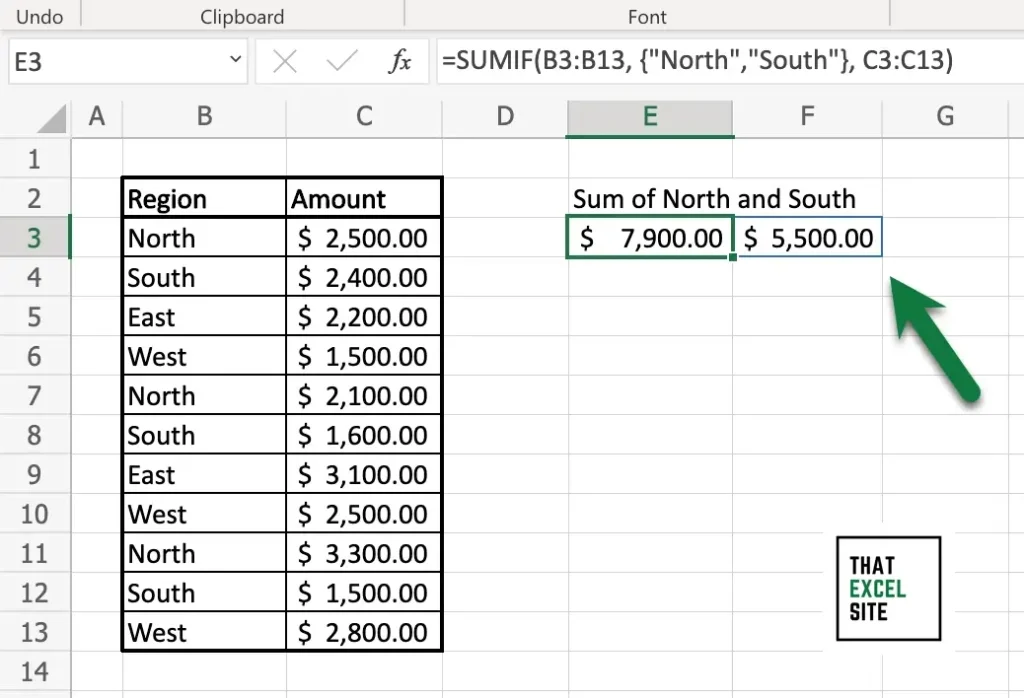
We can see that by using the function, Excel returns two cells of data. In this case, the values of $7,900 and $5,500 are returned. The values are wrapped in a blue border, meaning that they are part of a spill-over array. While this does tell us the sum that meet the different conditions, it doesn’t provide a single value.

Let’s see how we can wrap the SUMIF() function in the SUM() function to provide the sum of all cells that meet any of the conditions.

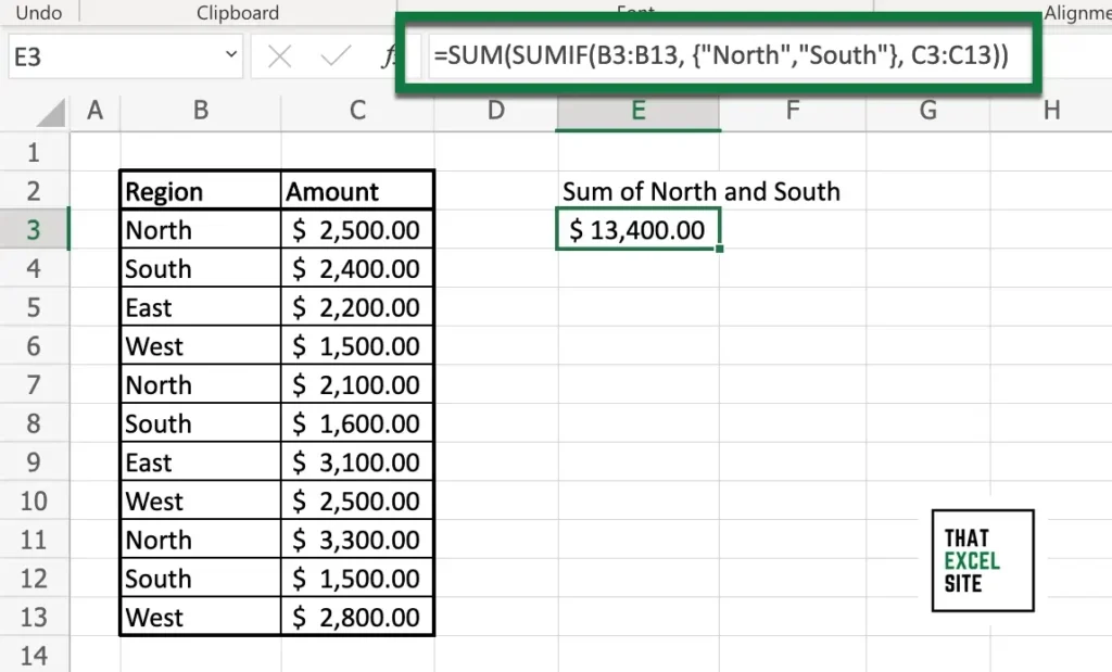
In the example above, we wrapped the function in the SUM() function, using the formula below:

=SUM(SUMIF(B3:B13, {"North","South"}))

By wrapping the SUMIF() function in the SUM() function, the function returns only a single value. This value represents the sum of all the cells meeting the given conditions, using OR logic.

How to Ignore #N/A Error in Excel SUMIF()

When adding values that contain an #N/A error, Excel will raise an #N/A. In order to ignore the #N/A error when using the SUMIF() function in Excel, you can use the criteria of “<>#N/A”. This ignores any cell that contains the #N/A in Excel, regardless of what’s causing it.

Because the function allows you to add values conditionally, we can easily instruct Excel to ignore cells that contain the error. Let’s see how we can use the SUMIF() function to resolve the error that occurs when adding values that contain a #N/A error:

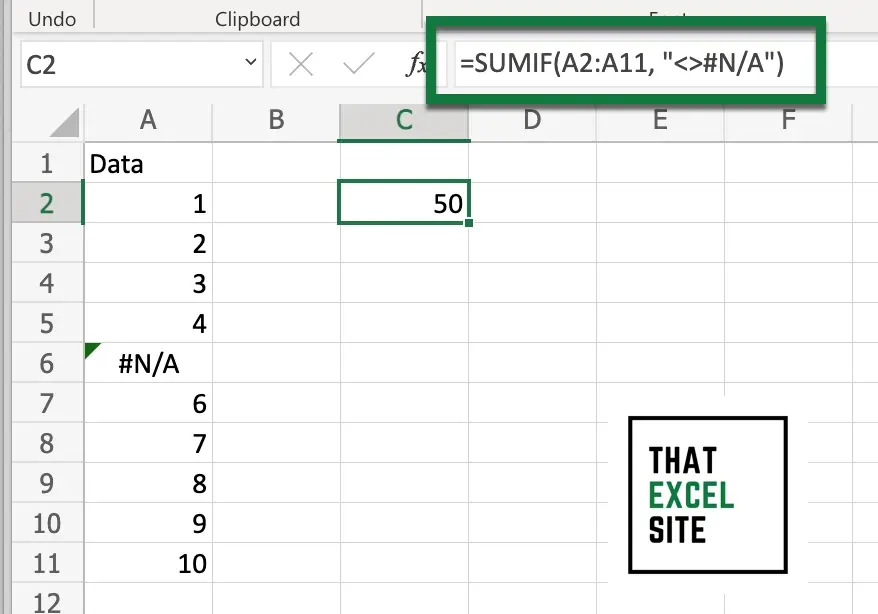
We can see that by using the following formula, the function no longer raises an error when summing values containing an #N/A error:

=SUMIF(A2:A11, "<>#N/A")

By using the formula above, you’re able to resolve errors caused by adding up values containing the Excel #N/A error.

Common Problems When Working with Excel SUMIF()

When working with the SUMIF() function, you may encounter some problems. There are two main types of problems that you may run into when working with the function:

1. No counts are returned when there should be. In order to resolve this, you should check if your conditions are wrapped in quotes, in order to close off the condition.
2. A #VALUE error is returned. If you’re referencing a value in another workbook, you need to make sure that the workbook is open. Excel expects that the workbook is open to be able to search within it.

The list above covers the main causes of problems when working with the function. Writing the criteria can be a bit awkward and can take some getting used to. Refer back to the table above to see how best to write your criteria.

Best Practices When Working with Excel SUMIF()

In this section, we’ll explore some of the best practices when working with the SUMIF() function. You can also think of some of these as tips and tricks that simply make the function more intuitive. Let’s dive right in!

SUMIF() is Case Insensitive

The SUMIF() function ignores casing, meaning that it doesn’t matter if your text is uppercase or lowercase. This can lead to some unexpected behavior, but can actually also make your function much simpler to use! For example, if you’re searching for North, it doesn’t matter if you search for NORTH, North, north, or even NoRtH! When you’re working with text data, the values may have some data entry errors. Because of this, text insensitivity can actually be quite helpful.

Named Ranges Make SUMIF() More Intuitive

Using named ranges can make working with the function significantly easier. Rather than using cell references and needing to worry about absolute references, using named ranges can make the function much simpler. If you think of the function of asking Excel to look in a certain range for certain criteria, this makes even more sense. Keep in mind that you’re also writing your function to be easily understood by future users of your workbook.

SUMIF() Works with “?” and “*” Wildcards

Using wildcards can make your criteria much stronger. Excel provides two wildcards that you can use in the SUMIF() function: ? replaces any single character, while * replaces any number of characters. Knowing this can make counting different string values that much easier.

Additional Resources for the Excel SUMIF() Function

To learn more about related topics, check out the resources below:

• Excel SUMIFS(): How to Use the Excel SUMIFS() Function
• How to Use Excel SUMIF() When Not Equal To Value
• How to Ignore #N/A Error in Excel SUMIF() (#DIV/0 etc.)
• How to Use Excel SUMIF() with Less Than Conditions
• How to Use Excel SUMIF() with Greater Than Conditions

Want to dive into the official documentation for the Excel SUMIF() function? Check it out here.