How to Ignore #N/A Error in Excel SUMIF() (#DIV/0 etc.)

The Excel SUMIF() function allows you to add values conditionally. However, it will also fail if you have a #N/A error, #DIV/0 error, or any other error in your range of data. Thankfully, this is quick and easy to solve! In this tutorial, you’ll learn how to ignore the #N/A error in the Excel SUMIF() function, as well as other errors such as the #DIV/0! error and #REF! error.

By the end of this tutorial, you’ll have learned the following:

• How to ignore #N/A errors in the Excel SUMIF() function, as well as other errors such as #DIV/0 and #REF!
• How to handle all errors when adding values using SUMIF() in Excel

Ignore #N/A Error in Excel SUMIF()

When you attempt to use the Excel SUM() function with a range of data that contains an #N/A error, Excel will raise the same #N/A errors. This is because the function accepts only numeric values as inputs. Let’s take a look at an example of what this looks like:

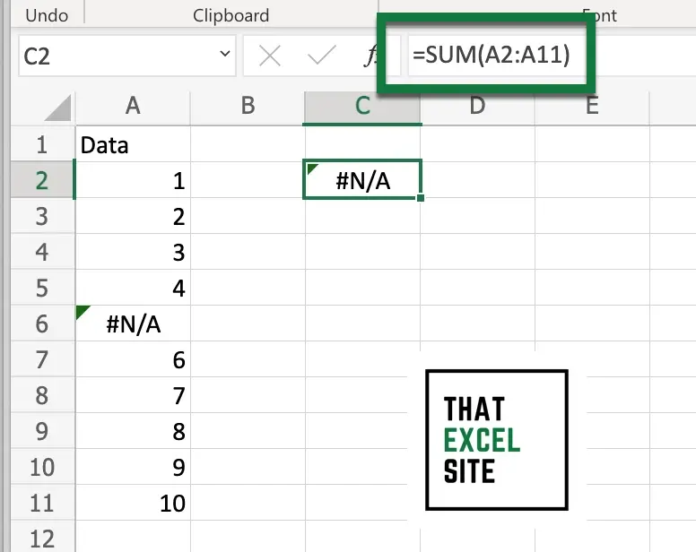
We can see in the example above that a #N/A error is raised when the SUM() function is used to add up values in a range that includes an error. In order to resolve this, we can simply use the Excel SUMIF() function. Because the function allows you to add values conditionally, we can easily instruct Excel to ignore cells that contain the error.

Let’s see how we can use the SUMIF() function to resolve the error:

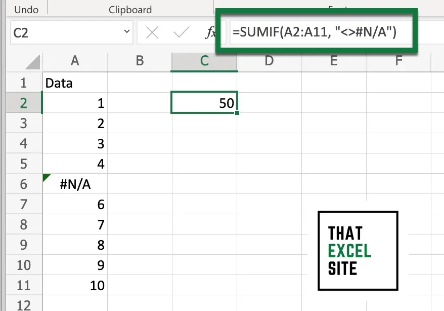
We can see that by using the following formula, the function no longer raises an error when summing values containing an #N/A error:

=SUMIF(A2:A11, "<>#N/A")

By using the formula above, you’re able to resolve errors caused by adding up values containing the Excel #N/A error.

Ignore #REF! Error in Excel SUMIF()

Similarly, we can use the Excel SUMIF() function to prevent errors caused by the #REF! error in Excel. The #REF! error is caused when a reference to a cell is no longer valid, such as when cells are deleted. In most cases, it’s best to investigate why the error is caused. However, you can use the SUMIF() function to ignore cells that contain the error.

Simply use the formula below to resolve the error:

=SUMIF(A2:A11, "<>#REF!")

Let’s take a look at an example of what this looks like:

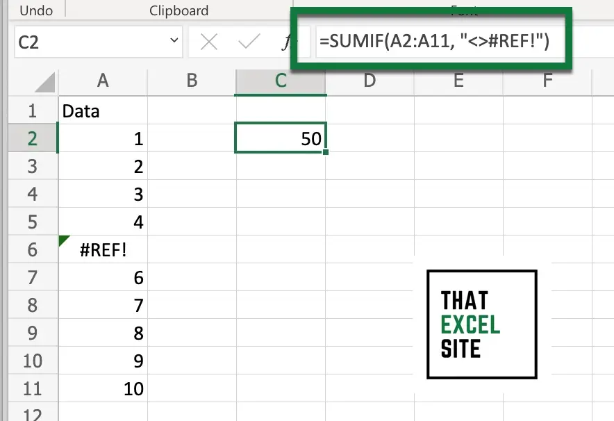
We can see that by using the SUMIF() function, we were able to add up values that contain the #REF! error.

Ignore #DIV/0 Error in Excel SUMIF()

Similarly, we can use the Excel SUMIF() function to prevent errors caused by the #DIV/0 error in Excel. The #DIV/0 error is caused when a value is divided by zero. Because dividing values by 0 is not possible, Excel correctly raises an error. You can use the SUMIF() function to ignore cells that contain the error.

Simply use the formula below to resolve the error:

=SUMIF(A2:A11, "<>#DIV/0")

Let’s take a look at an example of what this looks like:

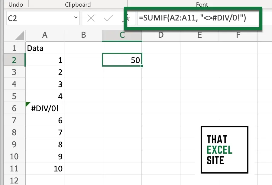
We can see that by using the SUMIF() function, we were able to add up values that contain the #DIV/0 error.

Ignore All Errors in Excel SUMIF()

In some cases, you may be working with ranges that contain multiple types of errors. In these cases, it’s easier to handle the errors using the IFERROR() function. The Excel IFERROR() function will assign a value to a cell if it contains an error. In this case, since we want to ignore the errors, we can assign the value of 0 as its fallback value.

Let’s take a look at the formula we can use to ignore all errors when adding values in Excel:

=SUM(IFERROR(A2:A11, 0))

Let’s take a look at an example of how this works:

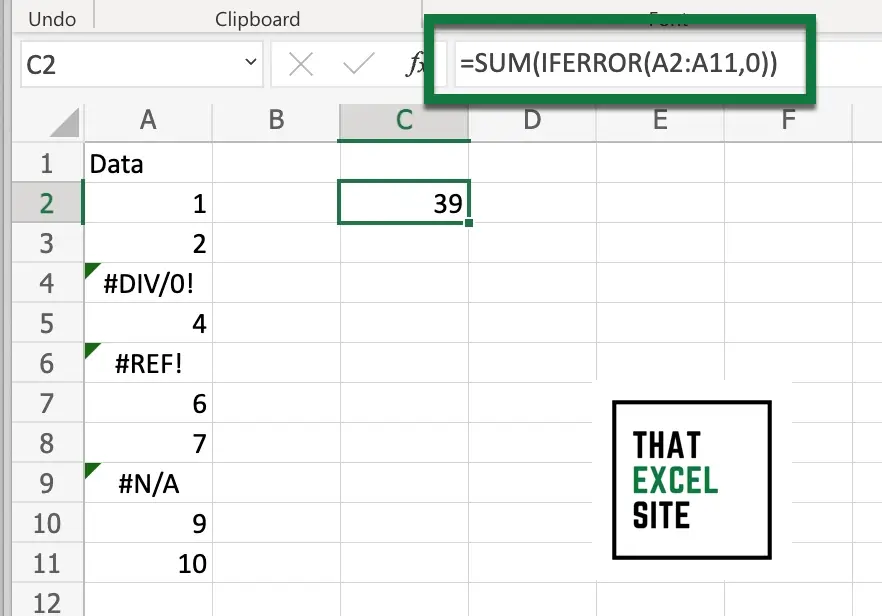
In this example, we can simply use the Excel SUM() function to add up all the values we need. This is because the IFERROR() function allowed us to convert all errors to 0. This essentially ignores any errors in the sum equation. It’s important to note that this may impact any additional calculations. For example, if you’re trying to calculate an average, you may want to calculate the average while ignoring zero values.

Conclusion

In this tutorial, you learned how to use the Excel SUMIF() function to ignore the #N/A, #REF!, and #DIV/0 errors. Because Excel errors indicate issues in your data, it’s often a good idea to investigate the error and resolve it at its source. However, this is not always possible. Being able to use the SUMIF() function to ignore these errors allows you to easily add up values that contain errors. You first learned how to use the SUMIF() function to handle each error individually. Then, you learned how to handle all Excel errors when adding values.

Additional Resources

To learn more about related topics, check out the tutorials below:

• Excel SUMIF(): How to Use the Excel SUMIF() Function
• Excel #REF! Error: What It Means and How to Fix It
• Excel #NUM! Error: What It Means and How to Fix it
• Excel #DIV/0 Error: What It Means and How to Fix it
• Excel SUMIF() Function: Official Documentation